Computing plays a vital part in the fabric of our daily lives. We engage with a wealth of sophisticated digital devices that play ever increasing roles in all aspects of our world: work and leisure, communication, socialisation, politics, economics, transportation, scientific research, genetics and even romance. Computing is woven deep into the fabric of daily experience; whether explicitly through smart phones and tablets or subtly buried within in our cars, fridges, coffee makers and central heating.  It is a trite and obvious truism to say that the internet has catapulted human society and technology into a brave new paradigm that is only in its early stages of a radical and ever-faster evolution.

Through our increasingly intimate experiences with computing devices, most people come to have some intuitive understanding of what a computer comprises and what it does in executing a computer program.  The modern computer would seem magical to anyone from a previous century.  How then did the concepts that underpin the modern digital computer arise? 

In this chapter we approach computation from a much more abstract perspective. We strip computation down to its fundamentals – what exactly is it and how can it be realised in the real world? In seeking to understand the difficulties and limitations of software engineering it is first important to understand what computation actually entails in a purely abstract and philosophical sense. Do we only find computation in networks of chips and wires or can it be realised in any suitably complex substrate – famously beer cans and windmills for example?

Algorithms

Before we get to computing per se  we first have to get to grips with the concept of an algorithm.  An algorithm is simply a well-defined set of simple steps which when performed in order will accomplish some specific end result.  The term algorithm describes any formal set of ordered rules that are guaranteed to achieve some specific (and desirable) transformation of an initial state into a new final state in a finite amount of time.  Think of an algorithm as a mindless, mechanical and foolproof recipe for achieving some result.

The word 'algorithm' itself is actually a Latinisation of the surname of the Muslim mathematician  Musa al-Khwarizmi; a scholar in the House of Wisdom in Baghdad. About 835 AD al-Khwarizmi wrote a  highly influential  book on arithmetical procedures – The Algebra. After translation into Latin, the corrupted version of his name – algorismus -  came to mean simply the "decimal number system".  This later became Anglicised as algorithm – meaning any well-defined mathematical function or procedure.

Algorithms then are not new and were well known to the Greeks.  The famous Sieve of Eratosthenes is a good example of a simple algorithm leaned by schoolchildren for finding all the prime numbers up to some limit.  Here is how it works:

To find all the prime numbers less than or equal to a given integer N:

1. Create a list of consecutive integers from 2 through N: (2, 3, 4, ...,N).

2. Initially, set a value P equal 2, the smallest prime number.

3. Delete  all multiples of  P from the list - these will be 2P, 3P, 4P, ..etc..; 

4. Find the next number in the list greater than P. If there was no such number, stop. Otherwise, set P to be this new number (which is the next prime), and repeat from step 3.

When the algorithm terminates, the numbers remaining are all the primes below N.

This algorithm is simple, repeatable, guaranteed to succeed and will also complete in a finite time for any value of N. Other examples of simple arithmetic algorithms are long division and multiplication. Even as schoolchildren, we are so familiar with these operations that we are unaware of the explicit sequence of steps and decisions we make in their execution. We are executing algorithms in our head.

All algorithms are characterised by the following fundamental properties:

1. Algorithms are independent of the medium within which the algorithm is implemented (substrate neutrality). The same algorithm (such as long division) may in principle be implemented with either paper and pencil, a mechanical calculating machine or a digital computer program. As long as the same steps are applied mindlessly and correctly the algorithm will succeed and generate the same result given the same starting data.  The power of the algorithm derives not from the physical materials used in its implementation from its inherent logical structure.

2. Once defined, algorithms are essentially mindless where each step requires no thought, insight or guiding intelligence to execute.  While complex algorithms do indeed require insight and intelligence to define, once specified the constituent steps may be applied by any mindless agent without further supervision.

3. An algorithm if correctly applied will always produce guaranteed results. It is a foolproof recipe if you like. 

4. A useful algorithm must deliver its result in some finite time – the algorithm must halt at some point and not run on indefinitely.

Algorithms are everywhere and are found across all sorts of domain, not just mathematics. The arrangement of matches in a knockout tennis tournament for example is an algorithm.  Your car sat-nav uses a complex algorithm to search a virtual map to find the optimal route. Every day billions of dollars in stock are traded by computerised algorithms on the global financial markets.  Facebook uses a complex algorithm to select content for your timeline. Perhaps the most globally significant and commercially valuable algorithm to date is the Google search engine. Updates to the Google page ranking algorithm strike terror into the hearts of webmasters everywhere and can have immense impacts on the commercial fortune of companies worldwide. 

Darwin’s dangerous idea of evolution by natural selection is yet another algorithm – albeit one without any defined goal or end point. As we shall see later, nature has discovered many heuristic tricks and tools which enable evolution to explore the vastness of biological design space in ways far more effective than blind search.

Given the idea of an algorithm, we can conceive computation as the process of manipulating symbols (representations) according to the rules of an algorithm.  But are all problems in arithmetic and mathematics for example soluble in terms of an algorithm? What then is computable?  

Functions

In mathematics a function is simply a relationship between some inputs (the function’s arguments) and an output (the value of the function). For example, addition and subtraction are simple functions. Each take two arguments (the numbers to be added or subtracted) and generate a definite value (the sum or difference of the arguments).

X + Y = Z       (addition)                                    X – Y = Z    (subtraction)

This notion of a function can be generalised for any number of arguments which are acted upon in some way to produce a related value. So examples would include the simple trigonometric functions (sine, cosine etc.), the exponentiation and logarithm functions, and also complex functions that might need five, six or more arguments.

Functions need not only work with numbers. Boolean logic (after the Irish logician George Boole) defines relationships between truth values, TRUE and FALSE. Boole defined a set of simple logical functions which relate truth values. For example, the AND logical function takes two truth value arguments and gives the result value TRUE only if both arguments are also TRUE. If either or both arguments are FALSE, the AND function gives the value FALSE. Similarly Boole defined other fundamental logical functions (OR, NOT, Exclusive-OR etc.)       

You can regard a function as a ‘black box’ whose inner workings are hidden. As long as the function delivers the correct result for the values of its arguments then the internal mechanism is irrelevant to the outside observer. But how do functions generate their output values? Perhaps the black box contains a genie able to magically summon up the correct result value by looking at the arguments. An alternative, but wildly less interesting, possibility is that the function may be realised in terms of an algorithm. Given the values of the input arguments, the algorithm performs a finite sequence of simple steps to generate a final result value.

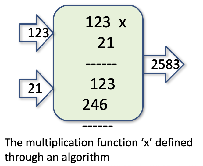
As an example, consider the multiplication function (*):    X * Y = Z 

This could be realised using the algorithm for long-form multiplication used by schoolchildren, e.g. 

This all seems very promising. But can every mathematical function be implemented in terms of an algorithm – some definite and finite sequence of simple logical steps? Such functions are said to be computable.  But are all functions computable? The answer to this goes right to the very soul of mathematics, as we shall see next. 

What Can Be Computed?

The start of the twentieth century  was a truly propitious time in human history. In the few years that followed both physics and mathematics would be transformed by major shifts in our understanding of reality. The development of general relativity and quantum mechanics occurred separately between 1900 and 1930 and these models radically changed our understanding of the very large and the very small. Just as Henry Ford  was pioneering ways of automating human labour within manufacturing, so mathematicians were beginning to think about the automation of human thought itself.

Mathematics at the start of the twentieth century was in a particularly reflective mood - reviewing the triumphs of the previous century and looking forward to the challenges of the next. The landscape of mathematics at the time was dominated by David Hilbert at Gottingen and in 1900 he convened an international conference of mathematicians in Paris. At the conference Hilbert presented a set of twenty-three currently unsolved problems in mathematics. Hilbert's problems ranged across the whole breadth of mathematics; from number theory through to topology, complex functions and elliptical geometry. 

Hilbert’s goal was to place mathematics on a sound and solid foundation. Could mathematics be based on a finite set of simple axioms from which, by a well-defined sequence of logical steps, all mathematical truths could be derived? Hilbert suggested that if a proposition can be expressed formally in the language of mathematics (specifically predicate logic) then there must exist some finite set of steps by which it can be shown either true or false. In other words, it should be able to establish the truth of any logical proposition by means of a finite and repeatable sequence of logical operations – an algorithm.  Could such a sequence of operations be performed in an automated way?

At a later conference in 1928, Hilbert condensed the fundamental issues underlying the foundations of mathematics into three key questions. Can the entirety of mathematics be expressed by a finite set of rules and axioms which are both complete and consistent?  If the ruleset is consistent then it must not contain any contradictions – a statement and its negation cannot both exist or be derivable within the system.  Furthermore, if the ruleset is complete, then all true statements must be provable totally within the fixed rules and axioms of the system. Finally, for any given statement in mathematics, must there necessarily exist some finite decision procedure – some algorithm – which will either prove the truth of the statement or its refutation, but never both? 

Within ten years all of Hilbert’s hopes for a final, complete and consistent basis for mathematics were dashed forever. In 1931 the brilliant Austrian logician Kurt Goedel proved that  any mathematics based on a closed set of axioms will always contain internal contradictions. No single mathematical system  complex enough to express the rules of arithmetic can ever prove its own consistency without introducing additional rules from outside the system.  There will always exist some paradoxical statement in the system – the so-called Goedel sentence – that is simultaneously both true and untrue. 

Such Goedel statements are self-referential and are analogous to the famous liar paradox. The proposition: ‘this sentence is false’ is paradoxically both true and false at the same time. If the system is expanded to resolve such problematic sentences  with additional axioms then a new Goedel sentence will arise and we are back to the same problem. Goedel proved that such systems are forever undecidable and thus mathematics itself is inconsistent.

The other question as to whether there must exist some finite decision procedure for any mathematical statement – known in German as the Entsheiddungsproblem – was fraught with difficulty. To begin to answer such a question there needs to be a more exact and rigorous definition of what a formal decision process is exactly. Also how it can be applied mindlessly and mechanically? 

The Turing Machine

It was the young Cambridge mathematician Alan Turing who conceived a brilliantly original and powerful line of thought. Familiar with the earlier work of Goedel, Turing became obsessed with the idea that there exist classes of mathematical problems unsolvable by any mechanical decision procedure. In other words, are there sound mathematical functions which are not computable?  (the un-computable numbers in Turing’s terminology).  Turing embarked on a quest to show the existence of non-computable functions, starting from his own first principles and following a wholly original line of thought.  Such a conjecture was unproven at the time and the solution would need the notion of “effectively calculable” to be more precisely defined. 

Turing asked himself: what is the simplest possible mechanism capable of performing any possible computation?  In answer he conceived a very simple device – he called it a ‘machine’ - capable of implementing a precise set of simple operations on some initial information to achieve some precise result. For example, such a machine would be able to generate the  product of any two numbers fed into it. In doing so the machine would be executing a specified algorithm for the desired process – long-form multiplication for example. The Turing Machine is not (necessarily) a real physical  device – it is purely an abstract thought experiment designed to illustrate a general and powerful principle about computation.

So how could such a device – now famously known as a Turing Machine -  operate?

A Turing Machine consists of four main components:

1. An infinite ‘tape’ divided into squares. Each square may be either blank or contain one of a finite number of symbols forming an alphabet. The simplest alphabet consists only of the symbols ‘0’ and ‘1’ for example.

2. A moveable  ‘scanner’ head which examines one square on the tape at any one time. The head may read the contents of the current square, may write a symbol from the alphabet into the current square, delete the symbol in the square or move one place (square) left or right on the tape.

3. A record of the current ‘state’ of the machine. The machine has a (small) finite number of states that may be in principle be simply labelled 1,2,3 ... etc.

4. A finite table of rules that completely defines the operation of the machine.

At the start, the tape consists of some set of symbols with the scanner head positioned at the start point and the machine in a given starting state.  For each discrete ‘step’ of the machine, the head reads the content of the current square and, given the current state number of the machine consults the book of rules as follows.

Each rule is of the form:

IF   in state M and the square contains  symbol  S THEN
  -  change the state to a new state M’ AND
  -  move the head LEFT or RIGHT or stay in the current square, AND
  -  perform one of the following operations:

• replace S with a new symbol S’ , OR

• delete the current symbol, OR

• do nothing, OR

• STOP

Instead of ‘state’ one could imagine the book of rules to consist of numbered pages; each page representing a single state of the machine. The rule book then tells the machine what to do for any given current symbol and then what page of the book to look at next.

Such a set of rules can easily be visualised as a simple lookup table with the following example form:

Given this simple set of equipment, the machine is capable of executing any correctly defined algorithm. Turing’s abstract machine captured the idea of operations occurring step by step in discrete time steps. Also important is the idea that the machine only has a finite number of states and operates upon a finite alphabet of symbols with a fixed number of rules.

Something rather similar to the Turing Machine exists within the nucleus of every living eukaryote cell. When the cell needs to express a new protein from one of the genes on its DNA it translates the gene into a strand of specially modified DNA called ‘messenger RNA’. A wonderful molecular machine called a ribosome then zips down the ‘tape’ of RNA, reading the chemical codes (three bases at a time) and assembling the appropriate amino acid for the current ‘symbol’. Strings of amino acids are assembled in the exact order required to create the specific protein molecule.  The assembled protein detaches and folds into the complex 3-dimensional shape that gives the specific protein (enzyme) its useful role in the cell metabolism. The ribosome and the RNA tape appear to behave in a similar way to the Turing Machine. In fact protein synthesis is a process of translation rather than computation.

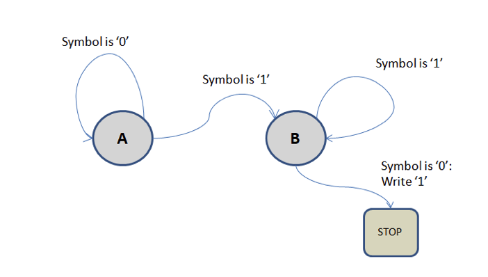
To show how simple and yet powerful a Turing Machine is, consider a TM that is able to add one to any number encoded on the tape.

Let the tape consist only of ‘1’s and ‘0’s. We can use unary notation (i.e. base 1) to represent any positive integer – the number N is simply N consecutive ‘1’s on the tape. Thus a tape containing 0001111000... represents the number 4.

The machine has only two possible states: A and B.  When a square is read the machine consults  its rule table and, depending upon whether in state A or B, performs an action depending upon whether the current square contains ‘0’ or ‘1’. 

The rule table is as follows:

        Symbol is ‘0’

       Symbol is ‘1’

If in state A

Move LEFT

Set State = B

Move LEFT

If in state B

Write ‘1’

STOP

Move LEFT

Suppose we start with the tape containing the number 3:  0011100

If we start in state A at the far right end of the tape, the machine will progress through the following steps (the current square is shown in bold):

0011100  

Move LEFT

0011100

Move LEFT

0011100  

Move LEFT, set state = B

0011100  

Move LEFT

0011100  

Move LEFT

0111100  

Write ‘1’ and STOP

Our tape now contains the number ‘4’ – we have added one to our original number.

Such a machine is incredibly clunky and tedious to perform such a boring and simple task. Consider adding ‘1’ to the number ‘103454464’? However, the example serves to illustrate the general principal that can be applied to any algorithm given some appropriate scheme for encoding information as a set of symbols on the tape.

In technical terms, a Turing Machine is an example of a Finite State Automaton which can alternatively be represented as a state transition diagram.  We simply draw each state of the machine as a circled node. For each state we draw arrows to the next possible states, labelling the arrow with the required current symbol and the action to be taken. A state may well have arrows that go back to the state itself, meaning ‘stay in the same state’. For our simple ‘add one’ machine the state diagram is simply the following: 

The Universal Turing Machine

To implement any specific algorithm though one would have to design the rule table and input tape for the exact task.  In other words, each algorithm needs a specific Turing Machine to be built for it. But what if it were possible to build a single Turing Machine that could perform any well-defined algorithm? Alan Turing’s next insight had huge and powerful implications for the future of automated computation.

Why not, said Turing, describe the rule table for a specific Turing Machine in some appropriate code that could then be written on to the input tape? The rule table code could then be followed by the input data required for the specific task (algorithm) in hand. A very special Turing Machine could then read in the rule table of the target Turing Machine and then, following its own rule table, could emulate the operation of the target Turing Machine. In effect, this generalised Turing Machine could implement ANY other possible Turing Machine. This then is the Universal Turing Machine – the UTM - a single machine able to execute any algorithm encoded as a ‘program’ on its input tape.  

All Turing Machines, and by their equivalence all computable functions, can be encoded as finite strings of symbols on a tape to be interpreted by the Universal Turing Machine. 

In conceiving his abstract machine, Turing had reduced potentially complex computations to a sequence of simple, mindless and mechanical steps – exactly the decision procedure required in Hilbert’s Entsheiddungsproblem. Once set in motion, the machine would proceed without error, step by step, and either run indefinitely in some loop of states or halt when it reached a  state that said STOP.

However, the key question that Turing had yet to prove was whether, given a specific Turing Machine definition, is it possible in advance (purely by inspection) to determine whether the machine will ever halt or run indefinitely.

What is the number of possible Turing Machines?  Since they must be able to be encoded as a finite sequence of symbols on a tape of the UTM then the number of possible Turing Machines must in principle be countable. But the number of possible mathematical functions is uncountable and, reasoned Turing, there must be valid mathematical functions that cannot be computable in terms of an equivalent Turing Machine. [These the are ‘uncomputable numbers’ of Turing’s seminal paper of 1936: ‘On Computable Numbers, With an Application to the Entscheidungsproblem’] 

Via a formal proof based upon the methodology of the Turing Machine and also logical techniques derived from Cantor and then Goedel, Turing succeeded in answering Hilbert’s fundamental conjecture. Hilbert was wrong: no mechanical procedure (algorithm or Turing Machine) can determine in a finite number of steps whether any mathematical function is provable or not.

Unknown to Turing, probably fortuitously for the future of computer science, the Entsheiddungsproblem was also being worked on by others with more mainstream approaches. Alonzo Church and Emil Post both independently developed novel proofs that the problem was unsolvable, and these were later shown to be exactly equivalent to Turing’s solution, albeit using very different mathematical tools.

While the work of Turing laid the formal foundations for modern computing, it is worth briefly mentioning a couple of earlier attempts at mechanical computation. 

The Jacquard Loom was invented by Joseph Marie Jacquard in 1804. Its novel innovation was to use a stack of  punched cards threaded together into a specific sequence. Each card contained rows of holes, each row corresponding to a row on the design. The card stack was feed into the loom where each sequential row controlled the movement of levers for the different colours of thread. In this way highly complex designs could be woven automatically with speed and accuracy. The loom then is an example of a single purpose stored program computer, although it was impossible to adapt its design for any other purpose, unlike the Universal Turning Machine.

In 1837 the English mathematician Charles Babbage proposed a design for a mechanical general purpose computing machine – the Analytical Engine. Based upon his earlier machine – the fixed-purpose Difference Engine – Babbage had conceived of a truly programmable machine able to perform any computation that could be defined as a sequence of simple operations.  Facing insuperable problems of precision machining and a chronic lack of money, the Analytical Engine was never completed. Babbage’s machine  critically lacked the elegant simplicity and philosophical power of the Turing Machine.

How then do we get from Turing’s powerful yet purely abstract and clunking machine to today’s sleek digital computers? Modern computers are called von Neumann machines after the pioneering work of the Hungarian polymath John von Neumann from 1945 onwards.  Von Neumann’s key innovation was to replace the 1-dimensional tape with a 2-dimensional random-access memory where each ‘square’ has a unique address and can be accessed immediately via this address. The von Neumann memory is like a 2-d matrix where each element has an X and a Y co-ordinate (address). Turing’s  idea of having to chunk through the tape square by square is now replaced by a single operation: go to square ‘X’ and perform operation ‘Y’.  

Modern von Neumann computers generally conform to the same generic architecture, whether a simple PC, a mobile phone or a complex parallel processing mainframe. A digital computer comprises a central processor (the microprocessor or CPU) together with a quantity of read-write memory. The memory consists of millions of locations where data (bytes comprising one’s and zero’s - bits) may be written and also read back. Each location in memory has a unique address through which it is accessed.  Each memory location stores a byte of information which may represent pure data (such as a numerical value, a pixel in an image or part of a sampled sound wave) or an instruction in part of a computer program.  Whether it stores data or an instruction code, the memory uses the same identical format.

A computer program is simply a sequence of coded instructions stored in memory; each instruction being a command for the CPU to perform some specific operation on data stored at some specific memory location. The CPU executes the program; reading and obeying each sequential instruction from the program stored in memory. In doing so it will read data from some parts of memory, manipulate it and write new data back to different locations in memory. 

Depending on the specific instructions of the program code, the computer can accomplish in general any information processing desired – whether a scientific calculation, filtering an image, sending and receiving messages, playing music or chess. The digital computer then is an efficient manifestation of Turing’s Universal Computing Machine - a truly general purpose computing device whose function and behaviour is defined solely by the software program fed into it. The underlying hardware remains unchanged regardless of which program is being executed. It is precisely this ability for universal computation that unlocks an almost infinite vista of possibilities that has shaped the fabric of our modern world.

The art or science of computer programming then can be reduced to the idea of finding the best Turing Machine in the space of possible Turing Machines. The concept of ‘best’ is immaterial – the fastest algorithm, the most accurate, the one using the least memory etc. But how large is the space of possible Turing Machines and how do we explore it efficiently to find the best, or ‘fittest’, candidate solution?  Furthermore, how do we find solutions (computer programs) which are adaptive and plastic rather than brittle and will not break catastrophically as things change?  

This is the topic of the next chapter.